500-Million Particle Pure Gravitational N-Body Simulation: Tidal Tail Structures from a Galaxy Collision This simulation is implemented using the pure N-body module of GASPHiA. The initial model was constructed with the open-source tool DICE, incorporating both a complete dark matter halo and a stellar disk component. The focus is on showcasing the process by which particles in the galactic disk evolve into characteristic tidal tails under gravitational perturbations during the interaction.
Why Consider Gravity?
In astrophysical SPH simulations, besides the impact process itself, the self-gravity of celestial bodies plays a crucial role in the final results. This also explains why we often do not introduce material strength models when simulating solid planet impacts, instead treating them as pure fluids. For some giant impact simulations, gravity not only requires real-time computation during the simulation but also demands solving the Poisson equation in the pre-processing stage to construct an initial celestial body in gravitational equilibrium before the impact calculation.
The gravity discussed here, namely self-gravity, refers to the mutual attractive force between SPH particles due to their mass distribution. This is entirely different from the gravity model used in hydrodynamic simulations (such as dam breaks) — the latter only needs to apply a uniform constant acceleration pointing toward the ground for each particle.
How to Compute Self-Gravity, and Why Do We Need a Tree Code?
In SPH simulations, computing self-gravity essentially means solving the gravitational force on each particle. According to Newton’s law of universal gravitation, any two particles exert a gravitational force on each other. For a system with $N$ particles, computing all pairwise interactions directly requires $O(N^2)$ operations. When the number of particles in astrophysical simulations reaches millions or even tens of millions, this direct summation approach becomes completely unacceptable in terms of computational cost.
This is the core motivation for introducing the Tree Code. The fundamental idea stems from a simple physical intuition: when a distant cluster of particles is far enough away, we don’t need to compute the contribution of each particle individually. Instead, we can approximate the entire cluster as a single equivalent mass point located at its center of mass. Through this approximation, the computational complexity can be dramatically reduced from $O(N^2)$ to $O(N\log N)$.
![Conceptual diagram of tree-based gravity computation, from reference [2]](/posts/gasphia/treecode/concept.png)
The Tree Code was first proposed by Barnes and Hut[1], so the tree structure based on their work is typically called the Barnes-Hut Tree. When implementing this data structure for CUDA architecture, GASPHiA draws from the parallel implementation approach in reference [2].
However, the method in reference [2] was designed for pure N-body simulations, where the data structure only needs to satisfy the requirements of self-gravity computation. In contrast, the SPH method not only needs to compute self-gravity but also relies on the tree structure for efficient neighbor particle searching. This fundamental difference in requirements leads to significant differences between GASPHiA’s final tree code structure and that in reference [2]. The specific differences are mainly reflected in two aspects: first, the management strategy for the number of child nodes in tree nodes; second, the warp voting mechanism during parallel tree traversal — reference [2] only needs to determine the condition for gravitational interaction, while GASPHiA, as an SPH code, must additionally integrate the logic for neighbor searching.
Despite these differences in implementation details, both approaches maintain a high degree of consistency in their core concept of spatial recursive partitioning. Therefore, readers can still use reference [2] as an important reference for understanding the underlying spatial partitioning logic.
Efficiency Comparison and Optimization
Background
Currently, GASPHiA has implemented self-gravity computation based on the Barnes-Hut Tree. However, compared to reference [2], during tree traversal, the lack of spatial sorting for particles means the efficiency is certainly not as high as with spatial sorting. To intuitively demonstrate the power of the Barnes-Hut Tree, we implemented brute-force pairwise self-gravity computation as a reference, and used the efficiency without spatial sorting as a baseline to explore the efficiency improvement after including the sorting process.
Computation Kernels
The tree-based self-gravity computation consists of the following kernels:
Reset Tree Structure
 1
 2
 3
 4
 5
 6
 7
 8
 9
10
11
12
13
14
15
16
void SPHOctree::resetOctree() { resetOctreeKernel<<<numBlocks, ThreadsPerBlock>>>( this->d_child, this->d_count, this->d_start, this->d_sorted, this->d_node_com_mass, this->d_node_hmax, this->d_mutex, this->d_node_index, this->num_particles, this->max_nodes); CUDA_CHECK(cudaGetLastError()); }Compute Particle Bounding Box
1
2
3
4
5
6
7
8
void SPHOctree::computeBoundingBox(RealType4 *d_particles) { computeMin(d_particles, d_reduceTmp, num_particles, d_bounding_box_min); computeMax(d_particles, d_reduceTmp, num_particles, d_bounding_box_max); CUDA_CHECK(cudaDeviceSynchronize()); CUDA_CHECK(cudaGetLastError()); }Build Tree Top-Down
 1
 2
 3
 4
 5
 6
 7
 8
 9
10
11
12
13
14
15
16
17
18
void SPHOctree::buildTree(RealType4 *d_positions) { buildTreeKernel<<<numBlocks, ThreadsPerBlock>>>( d_positions, this->d_node_com_mass, this->d_count, this->d_start, this->d_child, this->d_node_index, this->d_bounding_box_min, this->d_bounding_box_max, this->num_particles, this->max_nodes ); CUDA_CHECK(cudaGetLastError()); CUDA_CHECK(cudaDeviceSynchronize()); }Compute Center of Mass
 1
 2
 3
 4
 5
 6
 7
 8
 9
10
void SPHOctree::computeCenterOfMass() { computeCenterOfMassKernel<<<numBlocks, ThreadsPerBlock>>>( this->d_node_com_mass, this->d_node_index, this->num_particles); CUDA_CHECK(cudaGetLastError()); CUDA_CHECK(cudaDeviceSynchronize()); }Compute Self-Gravity
1 2 3 4 5 6 7 8 9 10computeGravityKernel<<<numBlocks, ThreadsPerBlock>>>( d_positions, this->d_node_com_mass, this->d_child, d_accelerations, this->d_bounding_box_min, this->d_bounding_box_max, this->num_particles, this->theta * this->theta, this->constG);
Performance Bottleneck Analysis
According to reference [2], the most time-consuming part of the entire tree code workflow is the final step — traversing the tree structure to compute self-gravity. The root cause lies in the mismatch between thread access patterns and data spatial distribution: if particle data is not explicitly sorted, particles within the same Warp may be far apart in physical space. This spatial distribution scatter directly leads to severe divergence among threads within a Warp when performing pruning decisions:
| |
When different particles in the same Warp face their respective target nodes, some threads may satisfy the pruning condition (mac_satisfied is true), while others still need to continue traversing deeper (false). Since CUDA’s Warp execution follows the single-instruction multiple-thread (SIMT) model, all threads must execute the same instruction path. Therefore, as long as any thread in the Warp does not satisfy the pruning condition — even if the majority could have terminated early — the entire Warp must enter the subsequent node drilling process. This execution path divergence caused by differences in data dependencies between threads greatly weakens the effectiveness of the pruning mechanism, causing substantial computational resources to be wasted on unnecessary deep node visits.
Performance Test and Comparison
To verify the above analysis, I first conducted a test: discretizing a cube to obtain regularly arranged particles, using single-precision computation with 1 million particles. The test results show that traversing the tree to compute gravity is indeed the most time-consuming step:
| |
Key finding: The time difference reaches 15x, and the only difference is whether particles are shuffled. Without shuffling, it is equivalent to having performed sorting (since the initial particle arrangement is regular); with shuffling, time skyrockets.
Detailed Profile data is as follows:
| Metric Name | Meaning | Regular | Shuffled |
|---|---|---|---|
| Elapsed Cycles | Total GPU clock cycles consumed by Kernel | ~0.29 Billion | ~2.58 Billion |
| Duration | Actual kernel runtime | ~0.19 s | ~3.10 s |
| SM Frequency | Average streaming multiprocessor frequency | ~1.55 GHz | ~830 MHz |
| Compute (SM) Throughput | Compute unit busyness | ~80.4% | ~79.2% |
| Memory Throughput | Overall memory subsystem busyness | ~61.5% | ~59.0% |
| L2 Cache Throughput | L2 cache access throughput | ~23.9% | ~14.1% |
| DRAM Throughput | VRAM direct access throughput | ~0.35% | ~15.7% |
| Achieved Occupancy | Actual active Warp ratio | ~98.6% | ~95.2% |
From the table, it is clear that after shuffling, L2 Cache Throughput drops from 23.9% to 14.1%, while DRAM Throughput increases from 0.35% to 15.7%. This demonstrates that particle sorting is crucial for improving data locality, fully utilizing L2 cache, and reducing direct VRAM access — directly causing the 15x performance difference.
Sorting Algorithm
The previous section’s shuffle experiment revealed that spatial locality plays a decisive role in implementing tree algorithms on CUDA. Better locality means that within a single Warp, the 32 threads are more likely to access the same tree nodes when traversing the octree, thereby greatly reducing Warp divergence and pushing L1/L2 cache hit rates to the limit, avoiding massive direct reads/writes to the slow DRAM.
Note: Although I used the expression “reduce Warp divergence (Warp Divergence)”, the threads are not actually diverging — they are simply opening too many nodes. In a sense, the inconsistency of
mac_satisfiedin warp voting is relatively strong. So I still borrowed the term “Warp divergence.”
However, in actual SPH or N-body simulations, as time progresses, particles violently collide and mix in space, and their indices in the memory array become completely decoupled from their real geometric positions. Therefore, we need to perform efficient spatial sorting after each frame’s tree construction.
1. Core Idea: Utilizing Natural Tree Topology Sorting
Since the octree itself is a perfect mesh partitioning of three-dimensional space, reading leaf nodes in the order of tree traversal (e.g., depth-first DFS or breadth-first BFS) yields a particle sequence clustered in three-dimensional space.
2. Gather Addressing Strategy: Sort Indices Only, Don’t Move Data
In a system with millions of particles, copying tens of megabytes of particle coordinates (float4 data) back and forth in global memory each time would not only be extremely time-consuming but also consume significant additional memory. We adopt the Gather addressing strategy:
- Do not move the actual particle positions in memory
- Generate a one-dimensional mapping array
sort sort[i]stores “the actual particle number that thread i should process”
During subsequent gravity computation, adjacent threads within the same Warp read adjacent values from the sort array. This way, particles processed by the same Warp are spatially close, and their tree traversal paths are also likely to be consistent.
3. Top-Down Sort
To complete sorting at extreme speed on the GPU, we utilize the count (subtree particle count) already computed during the tree-building phase, adopting a top-down parallel allocation mechanism. The parent node divides exclusive “memory intervals” for each child node in the sort array based on their count.
4. Profile Validation
Theoretically, after tree sorting and traversal, path divergence is further reduced because the parent nodes of particles in the same Warp are almost always together. To quantify this improvement, I reduced the particle count to 1 million and performed Profile analysis on the following three computation modes:
| Computation Mode | Description |
|---|---|
| 1. Fully Random | No tree sorting, particles randomly distributed in space |
| 2. Initial Regular | No tree sorting, particles regularly arranged in space |
| 3. Tree Sorting | Fully random but using tree sorting |
Profile command:
| |
Command parameter descriptions:
| Parameter | Meaning |
|---|---|
--set full | Collect all available performance metrics |
-f | Force overwrite existing output files |
-o profile/xxx | Specify output file path and name |
-k computeGravityKernel | Specify the Kernel name to Profile |
-s 2 | Skip the first 2 iterations after program startup before starting Profile (avoid cold start effects) |
-c 2 | Execute 2 repetitions and average (reduce measurement error) |
Comparison results:
| Computation Mode | Kernel Time | Executed Instructions | L1/TEX Hit Rate | Memory Throughput | Executed IPC | Warp Avg Instruction Cycles (CPI) |
|---|---|---|---|---|---|---|
| 1. Fully Random | 33.13 ms | 246.2 Billion | 48.23% | 2.37 GB/s | 2.97 | 13.75 cycles |
| 2. Initial Regular | 5.13 ms | 41.9 Billion | 57.52% | 8.14 GB/s | 2.99 | 13.44 cycles |
| 3. Tree Sorting | 3.11 ms | 22.1 Billion | 58.66% | 12.25 GB/s | 2.74 | 13.28 cycles |
From the results, tree sorting mode (3.11 ms) is approximately 10x faster than fully random mode (33.13 ms), and better than initial regular mode (5.13 ms). This proves that the spatial sorting strategy based on tree topology can significantly improve self-gravity computation efficiency.
Now, GASPHiA uses the code optimized with the tree sorting mode.
Performance Curves
The following two figures show the performance comparison of different computation modes across varying particle counts (linear and logarithmic scales):
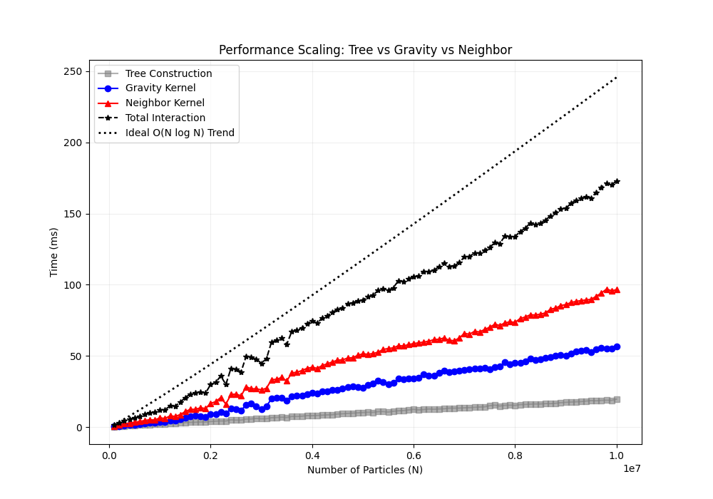
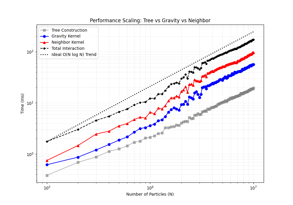
Note: In the figures above, “Build Tree” includes all processes such as bounding box computation and sorting. Compared to traversing trees for gravity or neighbor computation, the time for building the tree can be ignored.
Accuracy and Speedup Validation
I also tested the speedup and error of the Barnes-Hut algorithm relative to brute-force computation with 1 million particles. Note that the errors here are relative errors.
Performance and accuracy comparison across different $\theta$ parameters:
| $\theta$ | Computation Time (ms) | Max Relative Error | Avg Relative Error | Speedup |
|---|---|---|---|---|
| 0.1 | 181.877 | 0.00219153 | 3.27768e-05 | 7.42231x |
| 0.2 | 39.5222 | 0.00502609 | 6.86399e-05 | 34.1566x |
| 0.3 | 14.9356 | 0.0214612 | 0.00015996 | 90.3847x |
| 0.4 | 8.75622 | 0.0335255 | 0.00028779 | 154.17x |
| 0.5 | 5.88032 | 0.0711218 | 0.00053247 | 229.57x |
| 0.6 | 4.20147 | 0.0565245 | 0.000783245 | 321.303x |
| 0.7 | 3.52717 | 0.106591 | 0.00153542 | 382.728x |
| 0.8 | 3.21018 | 0.170889 | 0.002965 | 420.521x |
Accuracy validation figure:
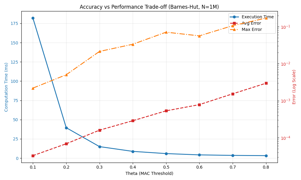
Conclusion: As $\theta$ increases, computational accuracy decreases (error increases), but computational speed significantly improves. At $\theta = 0.5$, we can achieve a 200x speedup while maintaining approximately 7% maximum relative error, making it a relatively ideal balance point.
References
[1] Barnes J, Hut P. A hierarchical O (N log N) force-calculation algorithm. nature. 1986 Dec 4;324(6096):446-9.
[2] Burtscher M, Pingali K. An efficient CUDA implementation of the tree-based barnes hut n-body algorithm. In GPU computing Gems Emerald edition 2011 Jan 1 (pp. 75-92). Morgan Kaufmann.