Implementation and Pitfalls of the P-alpha Porosity Model
In the animation of high-porosity pumice impact simulation (2.58 km/s), completely damaged particles are removed, and only kernel correction is enabled.
The animation above shows simulation results from GASPHiA of a projectile impacting a high-porosity pumice target at 2.58 km/s. The impact results are consistent with those given in the paper, demonstrating the accuracy of the damage model and P-alpha porosity model implementation in GASPHiA.
GASPHiA implements the P-alpha model described in the following two papers:
- Numerical simulations of impacts involving porous bodies I. Implementing sub-resolution porosity in a 3D SPH hydrocode
- Numerical simulations of impacts involving porous bodies: II. Comparison with laboratory experiments
Below is a note on the problems encountered during the implementation process.
1. Physical Problem Definition: P-alpha Model
In shock dynamics of porous materials (such as rubble piles and pumice), the macroscopic pressure $P$ satisfies the following relationship with the solid phase pressure $P_{\text{eos}}$ and porosity $\alpha$ (also called inflation factor):
$$P = \frac{P_{\text{eos}}(\rho_s, e)}{\alpha}$$where $\rho_s = \alpha \rho$ is the solid phase density, $\rho$ is the macroscopic density, and $e$ is the internal energy.
Note: $\alpha$ must be greater than 1. A value of 1 represents that the space represented by this particle has no voids.
Compaction Curve
The compression process of materials follows the compaction curve $\alpha_{\text{curve}}(P)$, defined as follows:
| Stage | Pressure Range | Formula |
|---|---|---|
| Elastic Stage | $P \le P_e$ | $\alpha = \alpha_0$ |
| Plastic Crushing Stage | $P_e < P < P_s$ | $\displaystyle \alpha = 1.0 + (\alpha_0 - 1.0) \left( \frac{P_s - P}{P_s - P_e} \right)^2$ |
| Full Compaction Stage | $P \ge P_s$ | $\alpha = 1.0$ |
Additionally, it should be noted that pore compaction is plastic and irreversible. If the theoretical $\alpha$ caused by the current pressure is greater than the historical minimum porosity $\alpha_{\text{old}}$, then take $\alpha = \alpha_{\text{old}}$.
2. Nonlinear Equation
We need to find an $\alpha$ that satisfies both the equation of state (EOS) generated pressure and lies on the compaction curve. Define the objective function:
$$F(\alpha) = \alpha - \min\left( \alpha_{\text{curve}}\left( \frac{P_{\text{eos}}(\alpha \rho, e)}{\alpha} \right), \alpha_{\text{old}} \right) = 0$$In the equation, $\alpha_{\text{curve}}$ refers to the compaction curve.
3. Bisection Method
The simplest and most intuitive approach is bisection, although it may take slightly longer execution time.
3.1 Iteration Count Analysis
Assume for a high-porosity material, the initial porosity $\alpha = 4$, corresponding to a physical porosity of $\phi = 1 - 1/\alpha$, which is 75%. If the final convergence accuracy required for iteration is:
$$\alpha_{n+1} - \alpha_n < \text{tol} = 10^{-12}$$Then in the worst case, iteration is needed:
$$n \ge \log_2 \left( \frac{L_0}{\text{tol}} \right) = \log_2 \left( \frac{4-1}{10^{-12}} \right)=42$$3.2 Accuracy Requirements
It is worth noting that EOS is extremely sensitive to density. In practice, it has been tested that tol must be less than 1e-7 to prevent artificial oscillations in the damage field. This is difficult to achieve for single-precision computation, so the porosity model in GASPHiA is forced to run in double precision, but when writing back, precision adjustment is performed to adapt to the overall computational workflow.
3.3 Performance Test Results
| |
| |
The execution time of solving EOS using the bisection method is unacceptable, as it is already comparable to the time for computing the right-hand side (single precision). We need an algorithm with faster convergence.
4. Newton-Raphson Method
The Newton-Raphson method is an efficient iterative algorithm for finding roots of nonlinear equations. For a general equation $f(x) = 0$, assuming we know its approximate root $x_n$ and the derivative $f’(x_n) \neq 0$, this method draws a tangent to the curve at $(x_n, f(x_n))$ and uses the intersection of the tangent with the x-axis as the next approximate root. The standard iteration formula is:
$$x_{n+1} = x_n - \frac{f(x_n)}{f'(x_n)}$$Newton’s method has the excellent property of second-order convergence near the root, meaning the number of significant digits approximately doubles with each iteration, and the convergence speed is much faster than the bisection method.
Returning to our porosity model, the objective equation to solve is $F(\alpha) = 0$, so the corresponding Newton iteration formula is:
$$\alpha_{k+1} = \alpha_k - \frac{F(\alpha_k)}{F'(\alpha_k)}$$To implement this iteration process, the core lies in calculating the nonlinear derivative of the objective function with respect to porosity $F’(\alpha) = \frac{dF}{d\alpha}$. Using the chain rule to expand it:
$$\frac{dF}{d\alpha} = 1 - \frac{d\alpha_{\text{curve}}}{dP} \cdot \frac{dP}{d\alpha}$$4.1 Derivative of Compaction Curve $\displaystyle \frac{d\alpha_{\text{curve}}}{dP}$
| Stage | Derivative |
|---|---|
| Elastic or full compaction stage, or in unloading state ($\alpha_{\text{curve}} > \alpha_{\text{old}}$) | $\displaystyle \frac{d\alpha_{\text{curve}}}{dP} = 0$ |
| In plastic crushing stage and in loading state | $\displaystyle \frac{d\alpha_{\text{curve}}}{dP} = -2 \frac{(\alpha_0 - 1.0)(P_s - P)}{(P_s - P_e)^2}$ |
4.2 Derivative of Pressure with Respect to Porosity $\displaystyle \frac{dP}{d\alpha}$
Given $P = \frac{P_{\text{eos}}(\alpha \rho, e)}{\alpha}$, taking the derivative with respect to $\alpha$:
$$\frac{dP}{d\alpha} = \frac{\alpha \cdot \frac{d P_{\text{eos}}}{d\alpha} - P_{\text{eos}}}{\alpha^2}$$According to the chain rule, $\frac{d P_{\text{eos}}}{d\alpha} = \frac{\partial P_{\text{eos}}}{\partial \rho_s} \cdot \frac{d \rho_s}{d\alpha} = \frac{\partial P_{\text{eos}}}{\partial \rho_s} \cdot \rho$.
Define $\frac{\partial P_{\text{eos}}}{\partial \rho_s}$ as dpdrho (provided directly by the Tillotson EOS), then:
5. Challenges Encountered: Oscillation
At the moment of impact, particles may be near physical boundaries (such as the elastic limit $P_e$).
5.1 Problem Description
- Loading step: High pressure $\to$ large derivative $\to$ Newton step too large $\to$ crosses the boundary into the unloading region.
- Unloading step: Enters unloading region $\to$ derivative suddenly becomes 0 $\to$ correction step bounces back to loading region.
This change caused by discontinuous derivatives results in Newton’s method cycling infinitely between two points and failing to converge.
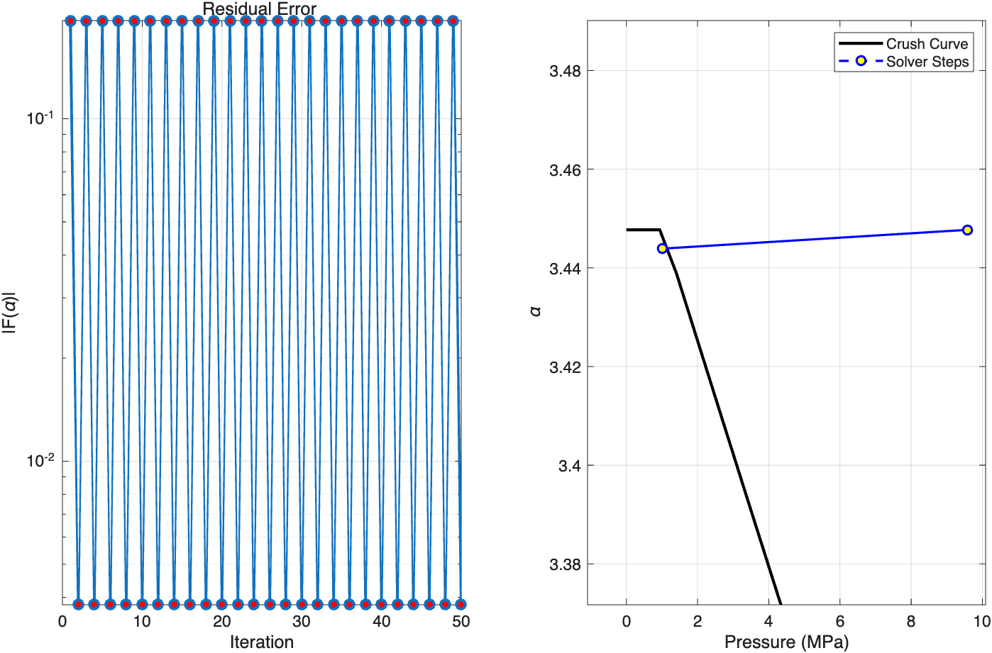
The figure shows the situation where, in the early stage of simulation, some particles, after receiving a slight amount of pressure, the Newton iteration oscillates and cannot converge.
6. Solution: Safe Newton Method
To balance the speed of Newton’s method with the stability of the bisection method, a hybrid algorithm with dynamic interval shrinking is introduced.
6.1 Algorithm Logic
| Step | Operation |
|---|---|
| 1 | Maintain interval: Initialize the safe interval $[a, b] = [1.0, \alpha_{\text{old}}]$ |
| 2 | Interval tightening: If $F(\alpha_k) > 0$, set $b = \alpha_k$; if $F(\alpha_k) < 0$, set $a = \alpha_k$ |
| 3 | Decision interception: Calculate the Newton step $\alpha_{\text{new}} = \alpha_k - \frac{F(\alpha_k)}{F’(\alpha_k)}$. If $\alpha_{\text{new}}$ falls outside the open interval $(a, b)$, it indicates Newton’s method has failed |
| 4 | Degradation handling: In this case, force the bisection method $\alpha_{\text{new}} = \frac{a + b}{2}$ |
| 5 | Fallback strategy: If Newton’s method fails to find a solution within the specified iteration steps, the solver will call the bisection method to solve |
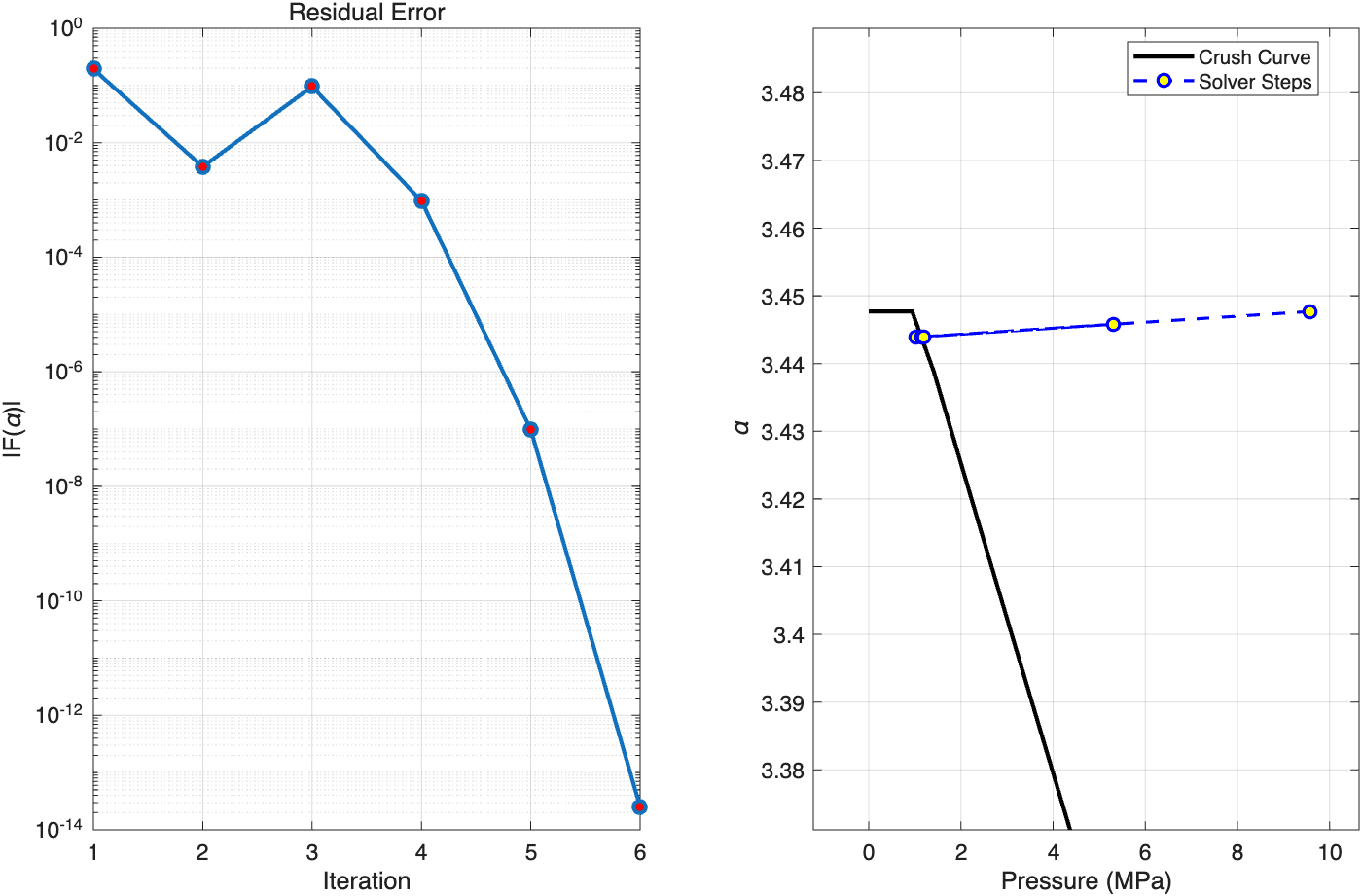
Under the same initial conditions, compared to the oscillation situation, the solver can now accurately jump out of the oscillation interval and find the solution.
6.2 Performance Comparison
In terms of efficiency, it is ten times faster than the bisection method at around 2.8ms. Compared to the execution time of the SPH right-hand side function at around 2.4ms, the EOS now only takes one-tenth of that time.
| |
| |
7. Final Results and Physical Verification
7.1 Compaction Curve Verification
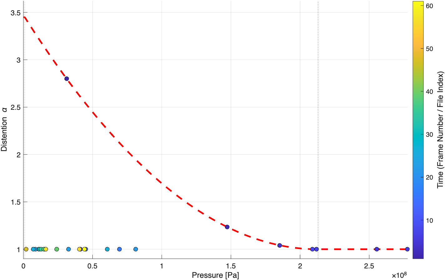
The red dashed line in the figure is the theoretical compaction curve, and the scattered points are the simulation output from GASPHiA. As time progresses, pressure causes proper pore compaction; after pressure is released, the porosity remains strictly unchanged, without any unphysical rebound phenomena. This fundamentally verifies that the irreversible logic implementation of the P-alpha model is completely accurate.
7.2 Macroscopic Experiment Comparison
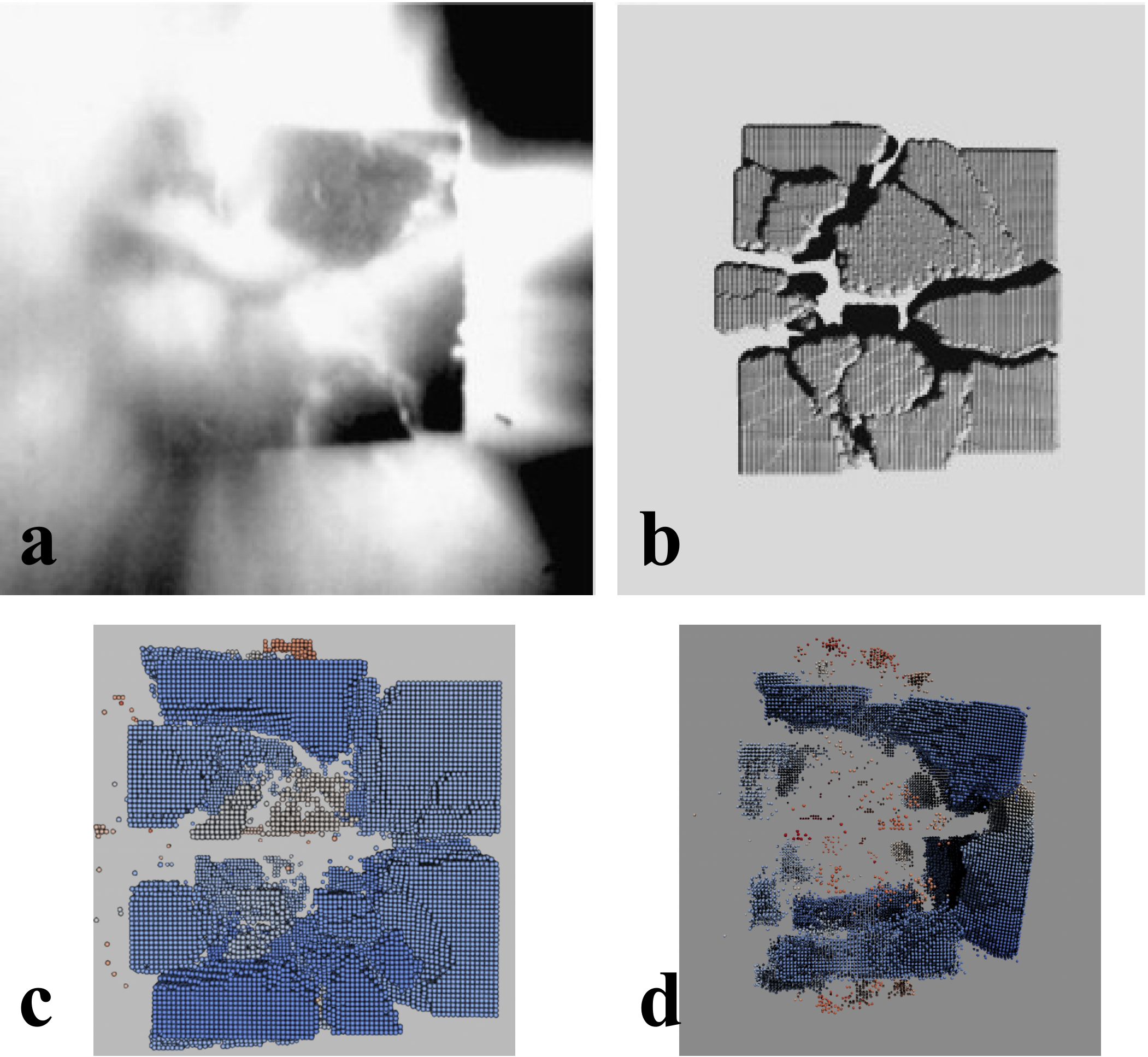
- Figures a, b: Experimental results and benchmark simulation results from Jutzi et al. 2009.
- Figure c: Simulation results from GASPHiA.
It can be seen that the physical morphology output by GASPHiA highly matches the original experiments and benchmark papers.
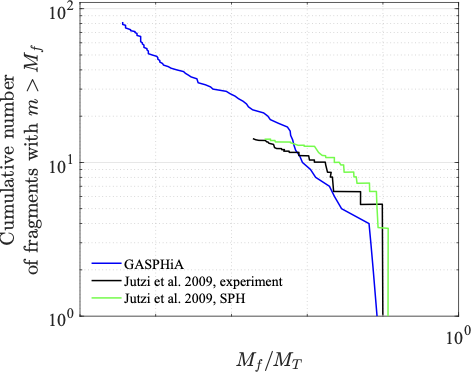
Post-process analysis of the impact results, extracting fragment cumulative mass distribution data:
The maximum residual fragment mass ratio calculated by GASPHiA is 11.67%, which has small error compared with the real experimental data of 9.96% given by the laboratory, further verifying the reliability of the core computational logic of the porous material solver.