1D Sod Shock Tube Experiment
TL;DR
This article presents a reproduction of the classic 1D Sod Shock Tube benchmark test using a custom-built CUDA SPH (Smoothed Particle Hydrodynamics) physics engine from scratch. The primary objective is to verify the engine’s capability to capture strong shock discontinuities. A critical numerical pitfall was identified and resolved: when handling initial step density fields, the traditional Continuity Density method causes severe non-physical oscillations, while the direct Summation Density demonstrates better robustness. In fact, continuity density is more suitable for high-speed impact problems.
1. Simulation Results
Comparison of two density calculation methods:
Summation Density (Success)

Continuity Density (Failure)

- Left (Success): Using summation density, the shock front, contact discontinuity, and rarefaction wave can be clearly observed propagating smoothly.
- Right (Failure): Using continuity density, oscillations appear at the initial density jump in the shock tube.
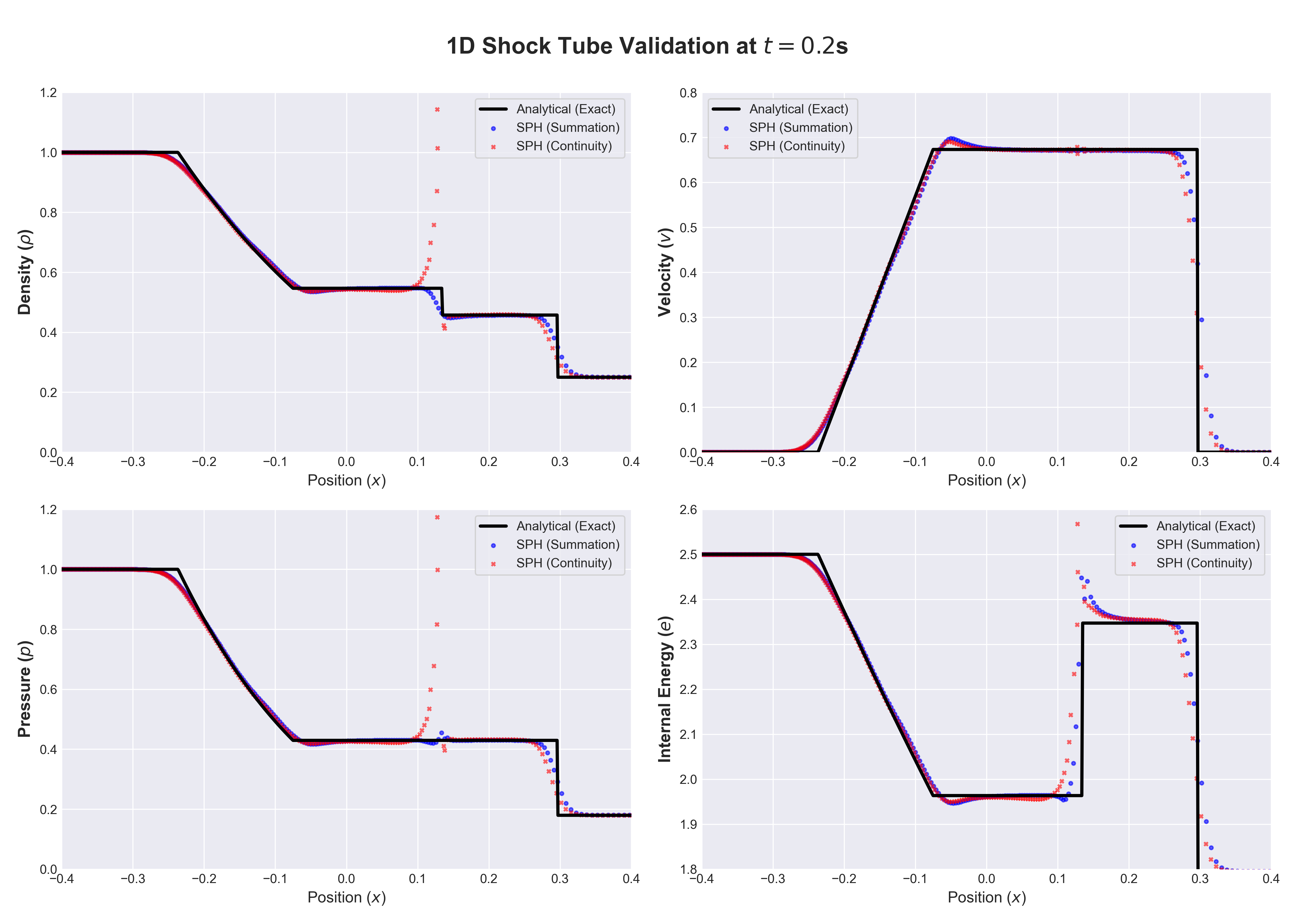
Figure 1: Density distribution comparison for the Sod shock tube. Shows the density along the x-direction at $t=0.2$ for three methods compared with the analytical solution. The red solid line is the analytical solution, blue dots are numerical results from the summation density method, and orange dots are numerical results from the continuity density method.
2. Problem Background
2.1 What is the Sod Shock Tube?
The Sod shock tube is a classic benchmark problem in fluid dynamics, used to verify numerical methods’ capability to capture shocks, contact discontinuities, and rarefaction waves. This problem simulates the instantaneous release of two gases at different states separated by a membrane in a one-dimensional tube.
2.2 Physical Model
This simulation uses the ideal gas model with the following governing equations:
Continuity Equation:
$$\frac{\partial \rho}{\partial t} + \nabla \cdot (\rho \mathbf{v}) = 0$$Momentum Equation:
$$\frac{\partial (\rho \mathbf{v})}{\partial t} + \nabla \cdot (\rho \mathbf{v} \otimes \mathbf{v}) = -\nabla p$$Energy Equation:
$$\frac{\partial (\rho e)}{\partial t} + \nabla \cdot (\rho e \mathbf{v}) = -p \nabla \cdot \mathbf{v}$$Equation of State (Ideal Gas):
$$p = (\gamma - 1) \rho e$$where $\gamma = 5/3$ is the adiabatic index.
3. Initial Conditions
At the initial time, the shock tube is divided into two regions by a membrane at $x=0$:
| Parameter | High Density Region (Left) | Low Density Region (Right) |
|---|---|---|
| Density $\rho$ | 1.0 | 0.25 |
| Velocity $v$ | 0.0 | 0.0 |
| Internal Energy $e$ | 2.5 | 1.795 |
| Particle Spacing $\Delta x$ | 0.001875 | 0.0075 |
| Smoothing Length $h$ | 0.01 | 0.01 |
| Region Range | $[-1.2, 0)$ | $(0, 1.2]$ |
| Number of Particles | 640 | 160 |
Total Particles: 800
The initial conditions set the left side as a high-pressure, high-density region and the right side as a low-pressure, low-density region. After the membrane is removed, the high-pressure gas on the left accelerates to the right, forming three wave structures: shock, contact discontinuity, and rarefaction wave.
4. Numerical Methods
4.1 SPH Density Calculation Approaches
This benchmark compares two SPH density computation methods:
Method 1: Summation Density
$$\rho_i = \sum_j m_j W(r_{ij}, h)$$where $W(r, h)$ is the kernel function and $h$ is the smoothing length. This method directly sums the masses of neighboring particles with clear physical meaning.
Method 2: Continuity Density
$$\frac{d\rho_i}{dt} = \sum_j m_j (v_j - v_i) \cdot \nabla_i W(r_{ij}, h)$$This equation is derived from the divergence of the momentum equation and is theoretically equivalent to the continuity equation.
Future Work
- 2D/3D Dam Break Simulation
- Simulations with Material Strength
References
- Sod, G. A. (1978). A survey of several finite difference methods for systems of nonlinear hyperbolic conservation laws. Journal of Computational Physics, 27(1), 1-31.
- Monaghan, J. J. (1992). Smoothed particle hydrodynamics. Annual Review of Astronomy and Astrophysics, 30, 543-574.
- Liu, G. R., & Liu, M. B. (2003). Smoothed particle hydrodynamics: a meshfree particle method. World Scientific.